Project Report
Abstract
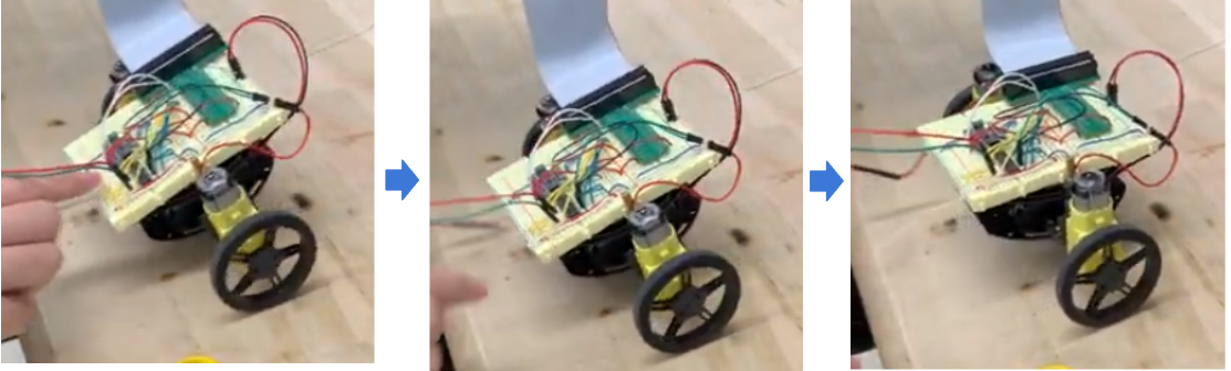
The goal of our final project is to create a self balancing two wheel robot. When pushed off balance, the robot will move forward and back to regain balance, which we define to be the upright position. We will use a PID control to control the angular velocity of the two wheels to achieve this capability. On Demo Day, visitors can push our robot and see it quickly return to the upright position.
Introduction / Project Motivation
Unlike their multi-wheeled counterparts, two wheeled robots are statically unstable. Unless the center of mass is perfectly placed or they experience a flat tire, two wheeled robots are doomed to fall one way or the other. This class of balancing vertically unstable objects can be broadly modeled by the inverted pendulum problem. Several interesting real world applications depend on solving the inverted pendulum problem, including launching and landing rockets and navigating the streets on a fancy Segway. In this project, we showcase how to stabilize a two wheeled robot using a PID controls algorithm. The block diagram of the system is showcased below in Figure 1 and the physical design of the robot is observable in Figure 2 and Figure 3.
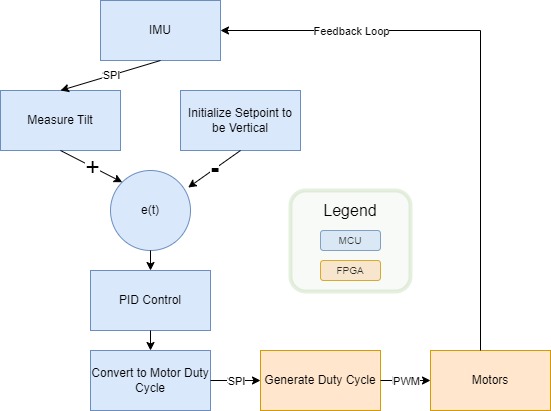
The control loop starts with the Microcontroller (MCU). It requests $y$ and $z$ acceleration data from an Inertial Measurement Unit (IMU) through SPI communication. Using this data, the MCU calculates the magnitude and direction of the robot’s tilt and passes this information to a PID control algorithm with the goal of minimizing the tilt magnitude. The control outputs are processed and sent to a Field Programmable Gate Array (FPGA) through SPI. The FPGA translates the desired control effort into PWM waves to appropriately spin the wheels of the robot. And the loop repeats.
Hardware
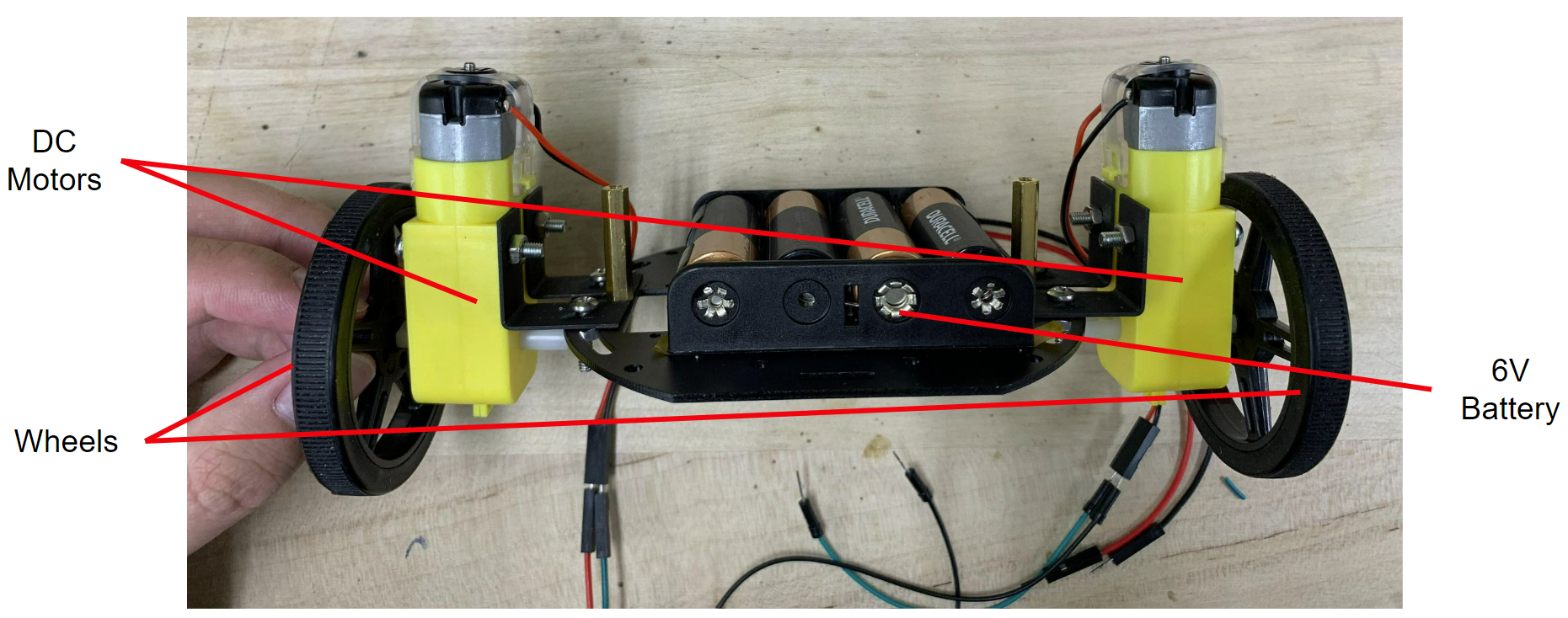
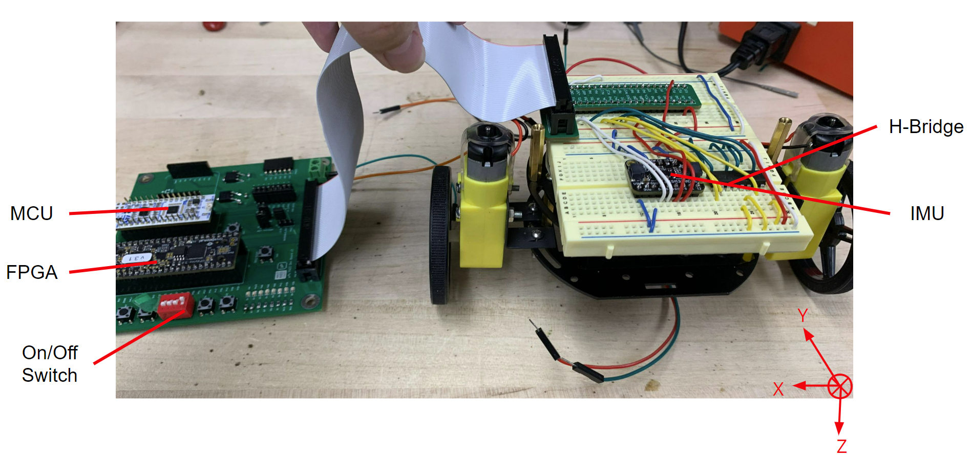
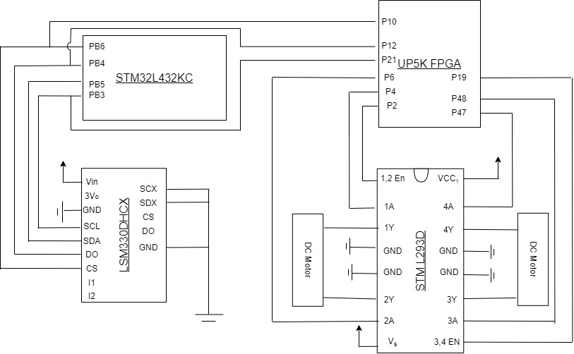
This project will incorporate an Inertial Measurement Unit (IMU), two DC motors, motor driver, and an external 6v battery.
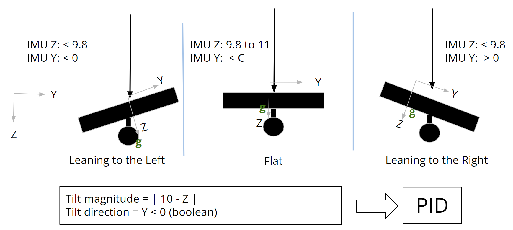
The IMU will provide measurements in six degrees of freedom ($x$, $y$, $z$, roll, pitch, and yaw). We will be using the IMU’s reported $y$ and $z$ accelerations to approximate the tilt of the robot. The tilt is measured from the way the gravitational force is decomposed in the $y$ and $z$ direction of the IMU. Note that the sensor’s positive $z$ direction points into the page and the positive $y$ direction points towards the front of the robot. When the sensor is flat, the $z$ axis lines up perfectly with the gravitational force vector and reports a value close to $g$. When the sensor is tilted at an angle, the effects of the gravitational force on the IMU’s $z$ axis decreases but increases along the $x$ and $y$ axes. We use the difference between the $z$ acceleration value and g to determine the magnitude of the tilt. Since the $y$ axis points towards the front of the robot, when the head of the robot is tilted downward, the IMU reports increasing positive $y$ acceleration. In the opposite direction, the IMU reports decreasing negative $y$ acceleration. We take the sign of the $y$ acceleration to differentiate between leaning forward and leaning backward.
We also use two brushed DC motors that can spin continuously and have one wire for power and one for ground. When connected to our motor driver (the L293D), we can control the spin of the motors bidirectionally. The L293D controls can control two motors independently. For each motor, it has two pins to control the spin direction of the motor (see FPGA section). Besides controlling the motors, the L293D allows us to amplify the current provided to the motors.
Finally, the whole system is powered by an external 6V battery. This extra battery provides necessary power to rotate the motors at higher speeds and allows our robot to be a self contained unit.
Schematics
MCU Design
The $\texttt{main}$ function located in spi.c consists of two functions $\texttt{init}$ and $\texttt{tim_loop}$.
In $\texttt{init}$ we initialize the SPI by making both $\texttt{phase}$ and $\texttt{polarity}$ to be 1. We configure the IMU and FPGA load and reset pins with $\texttt{GPIO_OUTPUT}$. We initialize timer 6 on the MCU which is used to keep track of the time step between IMU reads. Finally, we read the $\texttt{WhoAmI}$ register of the IMU, which contains a constant value. Comparing the value read from the IMU and the expected $\texttt{WhoAmI}$ value allows us to check the accuracy of our SPI communication.
In $\texttt{tim_loop}$ located in STM32L432KC_TIM.c contains the main code for our use of timer 6. We set $\texttt{Tim6}$ on the robot to count up to 20 milliseconds making the rate the IMU is read at to be about 50 Hz. In the timer loop there are two main parts:
- While the timer is counting, the MCU repeatedly reads the IMU and continually holds the most updated acceleration data.
- After the timer reaches the limit, the MCU computes the PID control based on the time step and the IMU data and then sends it to the FPGA through SPI.
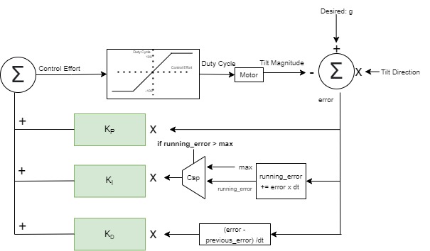
We implement a standard PID algorithm with a capped integral component. The input to the control loop is the tilt magnitude multiplied by the direction of tilt. The magnitude is calculated as $g$ - $z$ acceleration. The $\texttt{Hardware}$ section contains more information on how these values are calculated using IMU data. The proportional component acts directly based on the error. The integral component is proportional to a running sum of past errors. This sum is capped at $10$ to avoid excessive influence on the rest of the system. Without this cap, we found the robot was not able to respond quickly to changes in tilt. Finally, the derivative component is proportional to the difference between the current error and previous error. After calculating each component, we sum the values and apply a piecewise function to translate the control effort into an appropropiate duty cycle. The chosen function is linear ($y=x$) for control values from -100 to 100, and bounds the rest of the range to either -100 for negative control efforts or 100 for positive control efforts. See below for a block diagram of our PID algorithm.
FPGA Design
The top level module of our FPGA design takes in the inputs $\texttt{sck, clk, sdi, sdo, reset, and load}$ and controls 6 pins to control the H-Bridge. This module calls two modules, a $\texttt{SPI}$ module to load input from the MCU and a $\texttt{controller}$ module to generate a PWM signal.
The $\texttt{SPI}$ module takes in the inputs $\texttt{sck, load, sdi, and sdo}$ and the outputs the 2 bytes of information the MCU sends through SPI. When $\texttt{load}$ is pulled low, the module uses a shift register to hold the 16 bits. After $\texttt{load}$ is pulled high by the MCU, these 2 bytes of data are sent to the controller to generate the PWM signal.
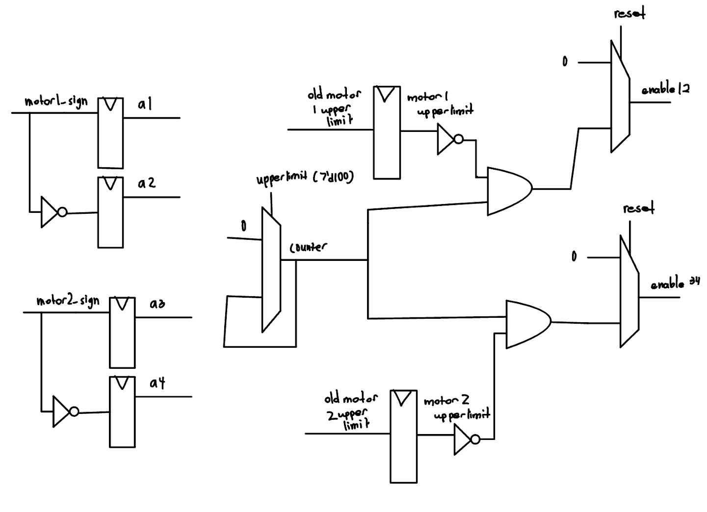
The $\texttt{controller}$ modules take in the 2 bytes of data and then pull 6 pins to generate a PWM signal. Each byte of data controlled one of the two motors. The below chart shows how the 2 bytes of information translated to the outputs shown in the H-Bridge Schematic
| $\texttt{motor1[8] (input)}$ | $\texttt{motor1 [7:0]}$ | $a_1$ (output) | $a_2$ (output) | $en_{1,2}$ (output) |
|---|---|---|---|---|
| 0 (forward) | value $\texttt{x}$ from (0, 100) | 1 | 0 | PWM signal, width = $\frac{\texttt{x}}{100}$ |
| 1 (backward) | value $\texttt{x}$ from (0, 100) | 0 | 1 | PWM signal, width = $\frac{\texttt{x}}{100}$ |
| $\texttt{motor2[8] (input)}$ | $\texttt{motor2 [7:0]}$ | $a_3$ (output) | $a_4$ (output) | $en_{3,4}$ (output) |
|---|---|---|---|---|
| 0 (forward) | value $\texttt{x}$ from (0, 100) | 1 | 0 | PWM signal, width = $\frac{\texttt{x}}{100}$ |
| 1 (backward) | value $\texttt{x}$ from (0, 100) | 0 | 1 | PWM signal, width = $\frac{\texttt{x}}{100}$ |
To create a PWM signal with width determined based on the input we used a variable $\texttt{counter}$ that repeatedly counted from 0 to 100. When $\texttt{reset}$ was high, we made sure pull both the enables low to make sure the robot did not move. However when $\texttt{reset}$ was low, we set the corresponding enable high whenever the $\texttt{counter}$ was less than the limit $\texttt{motorx[7:0]}$ and low when it was greater than the limit. This is illustrated in the below table,
| condition 1 | condition 2 | $\texttt{en}_{1,2}$(output) | $\texttt{en}_{3,4}$ (output) |
|---|---|---|---|
| $\texttt{counter} \leq \texttt{motor1[7:0]}$ | $\texttt{counter} \leq \texttt{motor2[7:0]}$ | 1 | 1 |
| $\texttt{counter} > \texttt{motor1[7:0]}$ | $\texttt{counter} \leq \texttt{motor2[7:0]}$ | 0 | 1 |
| $\texttt{counter} \leq \texttt{motor1[7:0]}$ | $\texttt{counter} >\texttt{motor2[7:0]}$ | 1 | 0 |
| $\texttt{counter} > \texttt{motor1[7:0]}$ | $\texttt{counter} > \texttt{motor2[7:0]}$ | 0 | 0 |
Results
We were able to successfully create PWM signals on the motor. The motor was able to spin in a range of speeds and in both directions. Furthermore we were able to communicate with the IMU, reading the expected value of the $\texttt{WhoAmI}$ register and get sensible accelerator data. This configuration allowed us to make sure we read and write correctly through SPI. Furthermore, we successfully used a clock on the MCU to make sure that our reads from the IMU were at a constant frequency to update the PID control algorithm.
However, there were some difficulties with the hardware design of the robot. As the chips and the battery pack together were too heavy for the robot to balance successfully, we decided to hold the chips in our hands. After this change, the robot showed a greater range of angles from which it can recover. Using a larger battery and wheels would also fix this issue.
Though the robot was able to regain balance after being pushed, we were unable to exactly tune the robot to minimize the oscillations. The robot takes a few seconds to recover from slight imbalances.